draw 3d plot in r
Make beautiful 3D plots in R — An Enhancement to the Storytelling
Examples along with data interpretation
![]()

Why data visualization? When nosotros piece of work with statistics, no affair what data we are processing, what models we are using, data visualization is always an inevitable part of the work. Sometimes nosotros might just make graphs mechanically and underestimate the importance of visualization. In fact, the visualization of the data not only makes the data easier to digest but too tells us more than than the data in text form and descriptive statistics. This is demonstrated past Anscombe's quartet.
Why 3D? Sometimes a 2D plot (or multiple of them) can contain enough information we need, just a 3D plot is usually more intuitive since the 3D space is where we reside. This is similar the 2D projection of a map, or atlas, which are what we usually see in geography textbooks, merely a earth is always more pleasant to utilize — more than fun, more intuition. Also, in statistics, we often see higher dimensional spaces (larger than 3 dimensions) and 3D visualization tin can help us with generalizing in college dimensional spaces.
In this article, some useful types of 3D plots will be introduced, namely, 3D surface plot, 3D line plot and 3D besprinkle plot, and they volition be implemented using libraries plotly or rgl. Likewise, we will accept a look at the estimation of the graphs — we should know what do the graphs mean since we are non just making nice pictures.
3D surface plot
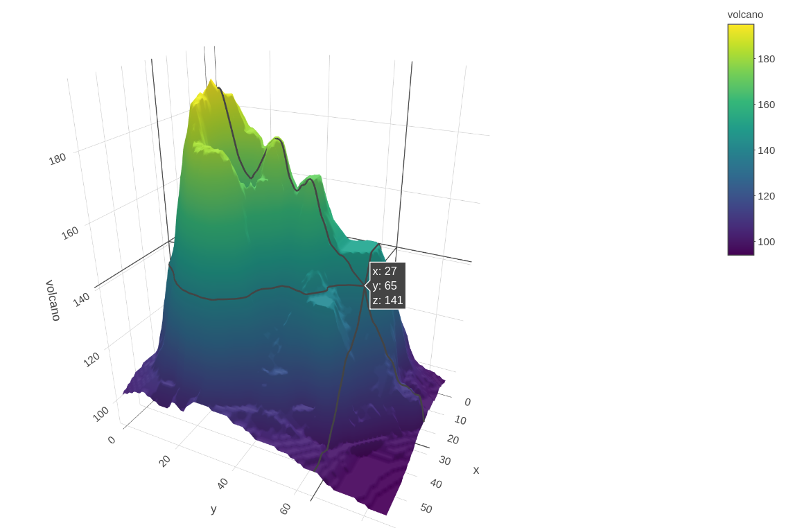
The 3D surface plot made using the plot_ly part in the plotly library is perfect for visualizing geographic information. Using the lawmaking snippet from the documentation we can draw a quite realistic volcano out of the built-in dataset volcano. This information is very easy to translate. The data set contains the topologic information on Auckland'south Maunga Whau Volcano, in the form of a 61 past 87 matrix. Each chemical element in the matrix is the acme of the volcano in a 10 by x filigree. Therefore, the result of the plot is the shape of the volcano. Not but the geographic data (elevation), but we can also use it to represent density, e.g. probability density. Firstly we generate a matrix of a probability distribution.
# simulate joint probability distribution (normal)
num.rows <- 60
num.cols <- 60 simulate <- role(north.row, n.col) {
# initiate the matrix
prob.n <- matrix(0, nrow=num.rows, ncol=num.cols)ten.seq <- seq(one, n.row)
y.seq <- seq(1, north.col)xx <- dnorm(x.seq, mean=n.row/2, sd=12)
for (i in i:n.row) {
y <- dnorm(i, hateful=n.row/2, sd=12)
res <- simulate(num.rows, num.cols)
prob.northward[i,] <- y * xx
}
prob.n;
}
In this instance, nosotros simulate a joint probability of two normally distributed independent variables. We can use the following code to plot the graph, which will output Figure ane.2 (a)
          # 3D plot of articulation probability distribution without project
fig.n <- plot_ly(z = ~res)
fig.northward <- fig.n %>% add_surface()
fig.n
Or nosotros can add projections to the x-z and y-z plane, this is set via the attribute profile.
          # add projection
fig.nc <- plot_ly(z = ~res,
            contours = listing(
            z = list(
            show=TRUE,
            usecolormap=Truthful,
            highlightcolor="#ff0000",
            project=list(z=True)
            ),
            y = list(
            bear witness=True,
            usecolormap=TRUE,
            highlightcolor="#ff0000",
            projection=list(y=Truthful)
            ),                     ten = list(
              evidence=True,
              usecolormap=TRUE,
              highlightcolor="#ff0000",
              project=list(x=TRUE)
              )
              )
              )
fig.nc <- fig.nc %>% add_surface()
fig.nc
The highlightcolor parameter determines the highlight color of the contours on the graph when hovering over the graph. In this instance, it's ready to be red. What does the graph tell us? The x and y axes announce the random variables Ten and Y, which accept normal distribution. The z-centrality shows the articulation probability of X and Y — the probability of X and Y taking on particular values (P(Ten=x and Y=y)), this determines the acme of the "hill" in Figure two.2. In our example, since X and Y are independent, P(10=x and Y=y) = P(X=ten)P(Y=y) according to the definition of independence. If X and Y have different standard deviations, one of the projections will be wider and the other will exist narrower, and the cross-section of the colina will exist an ellipse, instead of a circle.
Only we need to exist conscientious about the significant of the project on the x-z and y-z planes. It might seem like that they are marginal probabilities of X and Y, merely in fact, they are non. The projections only tell the states the corresponding value of P(X=ten and Y=y) with regard to X and Y. Withal, the marginal probability of X or Y should be the sum along rows or columns (recall well-nigh the table of marginal probability).
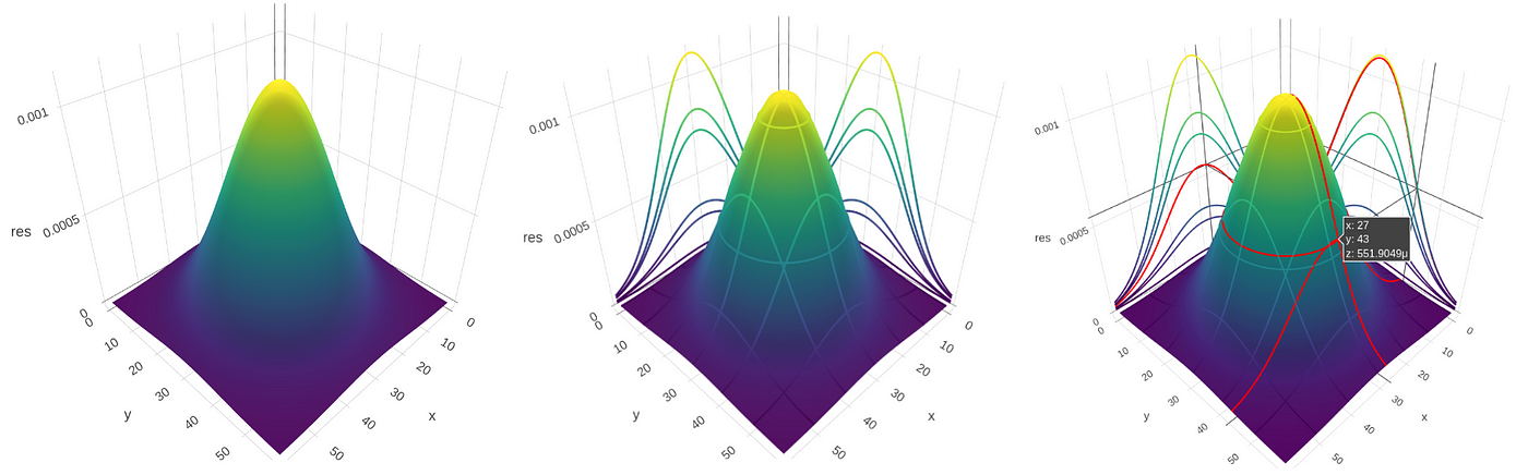
Also, we tin use a vector of color codes to define custom colors using the colors aspect. In Figure 1.3 the color templates are generated from coolors.
          colour.vec2 <- rev(c("#F2DC5D", "#F2A359", "#DB9065", "#A4031F", "#240B36"))
# color.vec2 <- rev(c("#F7AEF8", "#B388EB", "#8093F1", "#72DDF7", "#F4F4ED"))
fig.n2 <- plot_ly(z = ~res, colors=color.vec2)
fig.n2 <- fig.n2 %>% add_surface()
fig.n2 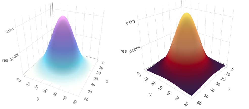
3d line plot and waterfall plot
3D line plots can be very useful when we desire to show multiple lines nicely. It enables united states of america to show multiple trends in ane graph, which saves the problem of designing more graphs and also adds to the aesthetic (this is a bit of personal stance). We utilise the electricity consumption data in the US as an case, the 3d line plot helps to demonstrate the trend of electricity usage co-ordinate to years and months in the same graph.
          # plot of the electricity usage in the Usa
data.united states <- usmelec
dmn <- list(month.abb, unique(flooring(time(data.us))))
# convert to data frame past month, to make information retrieval easier
res.us <- every bit.information.frame(t(matrix(data.usa, 12, dimnames = dmn)))          # set the values of the 3d vectors
north <- nrow(res.us)
10.us <- rep(month.abb, times=n)
y.u.s.a. <- rep(rownames(res.us), each=12)          z.us <- as.numeric(information.u.s.a.)
# nosotros need to append two values to the vector
# converted from the fourth dimension series and we let them
# equal to the concluding value in the time series and then the
# shape of the graph will non be influenced
n.z <- length(z.us)
z.us[n.z+1] = z.us[due north.z]
z.us[due north.z+2] = z.us[northward.z]          data.us <- data.frame(x.u.s., y.u.s., z.u.s.)
colnames(data.us) <- data.frame("ten", "y", "z")          fig.us <- plot_ly(information.usa, x = ~y, y = ~ten, z = ~z,
            type = 'scatter3d', mode = 'lines', color=~y.u.s.)
# to turn off the warning caused by the RColorBrewer
suppressWarnings(print(fig.us))
In this example, the data is stored every bit a time serial, which takes a chip of attempt to set up up the value of ten-, y- and z-axes. Fortunately, this is can be done merely using rep function.
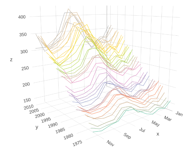
From the y-z plane, we tin can run into that from 1973 to 2010, people are mostly using more and more electricity, and from the x-z plane, we tin see how the electricity usage is distributed throughout the year (this is in fact and then-called seasonality, a very important property possessed by some time series).
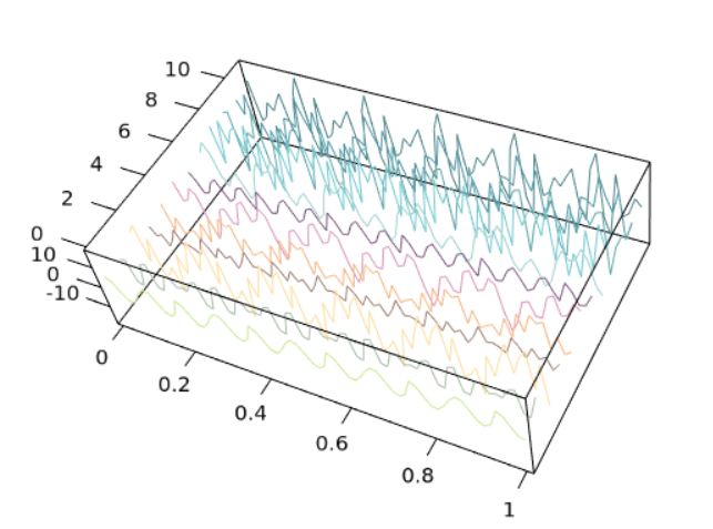
A waterfall plot (it's different from 3D line plots since in a 3D line plot there doesn't have to exist multiple lines — there tin can simply exist a single line going across 3D infinite) is a 3D plot, where multiple curves are shown simultaneously. Commonly, it is used to display spectra, e.g., to show the outcome of discrete Fourier transform. In R this can be realized using lines3d. The following code produces the plot of frequency components of a 10-element array later a complex Fourier transform.
          # For displaying the result
options(rgl.printRglwidget = TRUE)          x.f <- c(v, four.2, ix, three, 5.5, 8.2, 4.8, 6.iv, 11, ten.two, 8.nine, 10.9)
res.f <- fft(x.f)          nx <- length(x.f)
ny <- 70          xx <- seq(0, nx, by = ane)
yy <- seq(0, one, length = ny)          aspect3d(4, 2.5, 1)
axes3d()          cols <- c("#CBE896", "#AAC0AA", "#FCDFA6", "#A18276", "#F4B886", "#DD99BB", "#7F5A83", "#A1D2CE", "#78CAD2"
            , "#62A8AC", "#5497A7", "#50858B")
for (i in one:nx) {
            c <- ten.f[i]
            a <- Im(res.f[i])[1]
            b <- Re(res.f[i])[1]
            lines3d(yy, xx[i], c*(sin(a*xx) + cos(b*xx)), col=cols[i], lwd=ii)
}
The output of the above lawmaking is shown in Figure 2.two. For the code to run, the library rgl is necessary. Unlike the example before this (Figure 2.1), the lines are added one by one in a loop, instead of setting the locations of the points in the 3D space correct away.
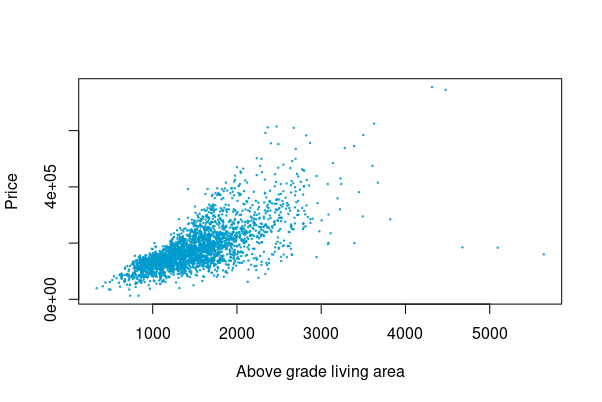
We can use waterfall plots to brandish density as well. This can be achieved past the office slicedens, which is available from the GitHub repository BivariateSlicer. We can utilize thesource role to import the whole source file right abroad, but some of the examples included might not run properly. Therefore, it'south better to only run the function. slicedens enables us to make slices in the information and present them in one 3D plot.
Nosotros apply the Ames Housing Dataset as an case, which is bachelor from Kaggle.
          housing <- read.csv2(file='data/AmesHousing.csv', header=Truthful, sep=',')
housing
summary(housing$Gr.Liv.Area)
footing <- housing$Gr.Liv.Area
cost <- housing$SalePrice          plot(ground, toll, cex=.two, col="deepskyblue3", xlab="Higher up grade living surface area", ylab="Price")          fcol <- c(.three, .viii, .8,.12)
lcol <- c(0.1, 0.five, 0.4,.1)
slicedens(ground,toll,
            fcol=fcol, bcol='white', lcol=lcol,
            gboost=0.015)
Expressed in a besprinkle plot, the data looks like Figure 2.4
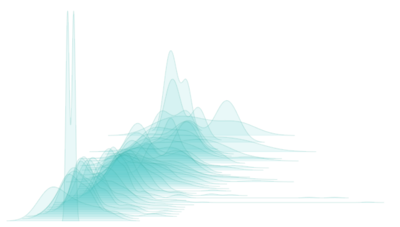
Imagine the scattered data is cut into several horizontal pieces, some of them contain more than points, some less. After arranging the slices into a single plot, the issue is displayed in Figure 2.5.
The plot in Figure 2.5 looks very nice, but this might not be the optimal fashion to present scatter data. We can see the density distribution from this figure of class simply compared with Figure 2.4, Figure two.5 doesn't seem to be so clear — we can't determine which surface area and the price range is nigh frequent. In this case, a 2D scatter plot like Effigy 2.four might be better. But because of the dainty visual effect and the interesting idea of slicedens, this 3D plot is also introduced in this commodity.
3d scattered plot
Besprinkle plots are a good mode of presenting discrete observations. Nosotros utilize Edgar Anderson's Iris data as an example, which gives the lengths and widths of sepal and petal of three species of iris. This is as well typically used for demonstrating PCA (Principal component assay). We volition use the following lawmaking to brand a scatter plot of the features of the flowers and the vectors of the components birthday. The code is a modified version of this. Don't worry if you don't know much most PCA, the math backside it will take some time to explain but the thought is simple — it is a technique that helps with reducing the number of dimensions of the dataset with minimum loss of information.
          # iris data
summary(iris)
iris$Species <- gene(iris$Species,
            levels = c("versicolor","virginica","setosa"))
pca <- princomp(iris[,ane:4], cor=Truthful, scores=TRUE)          # Scores
scores <- pca$scores
10 <- scores[,i]
y <- scores[,2]
z <- scores[,3]          # Loadings
loads <- pca$loadings          scale.loads <- 3          p <- plot_ly() %>%
            # the scatter plot of the data points
            add_trace(x=ten, y=y, z=z,
            blazon="scatter3d", mode="markers",
            marker = list(color=y,
            colorscale = c("#FFE1A1", "#683531"),
            opacity = 0.7, size=2))          ns <- rownames(loads)
# add the vectors of the components
for (k in one:nrow(loads)) {
            x <- c(0, loads[g,i])*calibration.loads
            y <- c(0, loads[k,2])*scale.loads
            z <- c(0, loads[g,3])*calibration.loads
            p <- p %>% add_trace(x=ten, y=y, z=z,
            type="scatter3d", fashion="lines",
            line = list(width=eight),
            opacity = 1, name=ns[k])
}
# display the graph
print(p)
A 3D scatter plot tin very well assistance the states see the distribution of the information and what office the "components" play.
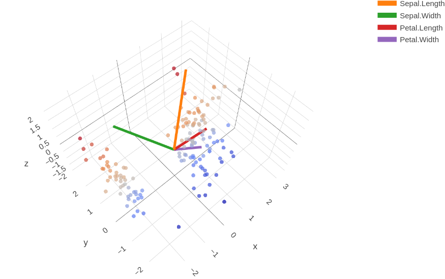
In Figure 3.1, the data is not clustered (colored by the species), the color just changes along the y-axis. To plot amassed data, we tin can exercise it using the office plot_ly very easily.
          p <- plot_ly(iris, x=~Sepal.Length, y=~Sepal.Width,
            z=~Petal.Length, color=~Species) %>%
            add_markers(size=ane)
print(p) 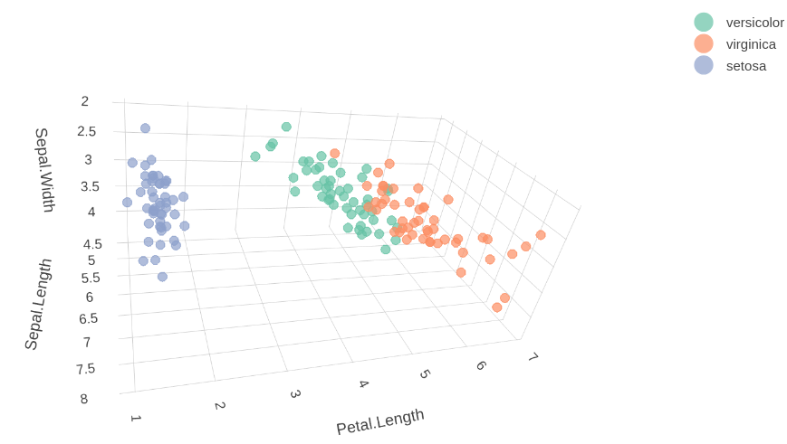
Other useful 3D plots
In this department, we introduce another plots with code available.
(1) The fancy 3D histograms from: http://www.sthda.com/english language/wiki/impressive-package-for-3d-and-4d-graph-r-software-and-data-visualization, which is a nice tool for displaying the frequency of detached information, due east.g. the number of seismic events with regard to longitude and latitude (Figure three.three). In Figure 3.3, the columns denote the counts of seismic events in each range of longitude and latitude (the small squares in the x-y plane). On the x-y plane beneath the grids, the projection is the scatter plot of the depths of the seismic events in the given ranges.
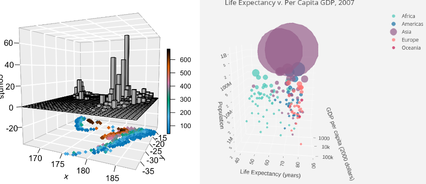
(2) The 3D bubble plot from: https://plotly.com/r/3d-scatter-plots/. Information technology can be used to show the relation of multiple variables in a single 3D plot. The example given in Effigy 3.4 shows the relationship betwixt population, life expectancy, GDP, and countries (the characterization of every marker, it is visible when hovered over) also as state sizes (the size of the markers).
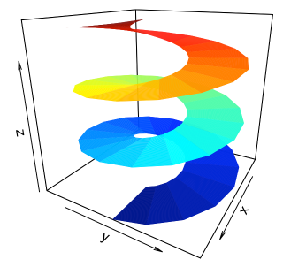
(3) 3D surface plots for developing geometric intuition from: https://rviews.rstudio.com/2020/12/xiv/plotting-surfaces-with-r/. The examples from this article are very practical for visualizing topological shapes.
Source: https://towardsdatascience.com/make-beautiful-3d-plots-in-r-an-enhancement-on-the-story-telling-613ddd11e98
0 Response to "draw 3d plot in r"
Post a Comment